
Super Resolution UNET
Contents
Super Resolution UNET#
This tutorial is available as an IPython notebook at malaya-speech/example/super-resolution-unet.
This module is language independent, so it save to use on different languages. Pretrained models trained on multilanguages.
This is an application of malaya-speech Pipeline, read more about malaya-speech Pipeline at malaya-speech/example/pipeline.
Dataset#
Trained on English, Manglish and Bahasa podcasts with augmented noises, gathered at https://github.com/huseinzol05/malaya-speech/tree/master/data/podcast
Purpose of this module to increase sample rate.
[1]:
import malaya_speech
import numpy as np
from malaya_speech import Pipeline
import IPython.display as ipd
[2]:
import logging
logging.basicConfig(level=logging.INFO)
List available UNET deep models#
[3]:
malaya_speech.super_resolution.available_unet()
INFO:malaya_speech.super_resolution:Only calculate SDR, ISR, SAR on voice sample. Higher is better.
[3]:
| Size (MB) | Quantized Size (MB) | SDR | ISR | SAR | |
|---|---|---|---|---|---|
| srgan-128 | 7.37 | 2.04 | 17.03345 | 22.330260 | 17.454372 |
| srgan-256 | 29.50 | 7.55 | 16.34558 | 22.067493 | 17.024390 |
We modified SRGAN to do 1D Convolution and use output distance as generator loss, originally use content loss.
Load UNET deep model#
def unet(model: str = 'srgan-256', quantized: bool = False, **kwargs):
"""
Load Super Resolution 4x deep learning UNET model.
Parameters
----------
model : str, optional (default='srgan-256')
Model architecture supported. Allowed values:
* ``'srgan-128'`` - srgan with 128 filter size and 16 residual blocks.
* ``'srgan-256'`` - srgan with 256 filter size and 16 residual blocks.
quantized : bool, optional (default=False)
if True, will load 8-bit quantized model.
Quantized model not necessary faster, totally depends on the machine.
Returns
-------
result : malaya_speech.model.tf.UNET1D class
"""
[4]:
model = malaya_speech.super_resolution.unet(model = 'srgan-256')
model_128 = malaya_speech.super_resolution.unet(model = 'srgan-128')
INFO:malaya_boilerplate.frozen_graph:running Users/huseinzolkepli/.cache/huggingface/hub using device /device:CPU:0
INFO:malaya_boilerplate.frozen_graph:running Users/huseinzolkepli/.cache/huggingface/hub using device /device:CPU:0
Load Quantized deep model#
To load 8-bit quantized model, simply pass quantized = True, default is False.
We can expect slightly accuracy drop from quantized model, and not necessary faster than normal 32-bit float model, totally depends on machine.
[5]:
quantized_model = malaya_speech.super_resolution.unet(model = 'srgan-256', quantized = True)
quantized_model_128 = malaya_speech.super_resolution.unet(model = 'srgan-128', quantized = True)
WARNING:malaya_boilerplate.huggingface:Load quantized model will cause accuracy drop.
INFO:malaya_boilerplate.frozen_graph:running Users/huseinzolkepli/.cache/huggingface/hub using device /device:CPU:0
WARNING:malaya_boilerplate.huggingface:Load quantized model will cause accuracy drop.
INFO:malaya_boilerplate.frozen_graph:running Users/huseinzolkepli/.cache/huggingface/hub using device /device:CPU:0
Important factor#
Currently we only supported 4x super resolution, if input sample rate is 16k, output will become 16k * 4.
We trained on 11025 for input sample rate, 44100 for output sample rate.
Predict#
def predict(self, input):
"""
Enhance inputs, will return waveform.
Parameters
----------
input: np.array
np.array or malaya_speech.model.frame.Frame.
Returns
-------
result: np.array
"""
Let say we have a low sample rate audio,
[6]:
sr = 44100
reduction_factor = 4
[10]:
original_y, _ = malaya_speech.load('speech/44k/test-0.wav', sr = sr)
original_y = original_y[: sr * 4]
len(original_y) / sr
[10]:
4.0
[14]:
y, sr_ = malaya_speech.load('speech/44k/test-0.wav', sr = sr // reduction_factor)
y = y[:sr_ * 4]
ipd.Audio(y, rate = sr_)
[14]:
[12]:
%%time
output_256 = model(y)
ipd.Audio(output_256, rate = sr)
CPU times: user 24.9 s, sys: 2.96 s, total: 27.8 s
Wall time: 5.26 s
[12]:
[13]:
%%time
output_128 = model_128(y)
ipd.Audio(output_128, rate = sr)
CPU times: user 7.57 s, sys: 1.45 s, total: 9.02 s
Wall time: 2 s
[13]:
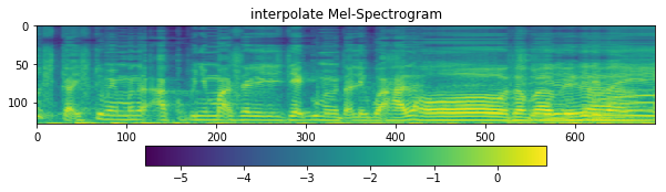
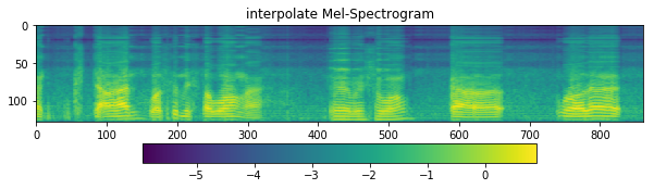
Below is common technique people do upsampling using interpolate,
[16]:
y_ = malaya_speech.resample(y, sr // reduction_factor, sr)
[17]:
import librosa
import matplotlib.pyplot as plt
[19]:
sampling_rate = 44100
fft_size = 2048
hop_size = 256
win_length = None
window = 'hann'
num_mels = 128
fmin = 0
fmax = None
mel_basis = librosa.filters.mel(
sr=sampling_rate,
n_fft=fft_size,
n_mels=num_mels,
fmin=fmin,
fmax=fmax,
)
[20]:
D = librosa.stft(
original_y,
n_fft=fft_size,
hop_length=hop_size,
win_length=win_length,
window=window,
pad_mode='reflect',
)
S, _ = librosa.magphase(D)
mel = np.log10(np.maximum(np.dot(mel_basis, S), 1e-10)).T
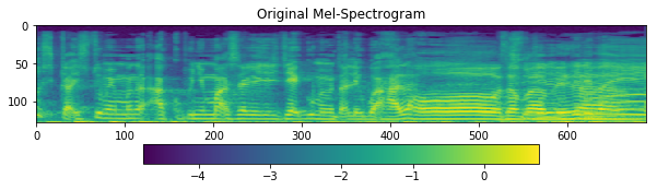
fig = plt.figure(figsize=(10, 8))
ax1 = fig.add_subplot(311)
ax1.set_title('Original Mel-Spectrogram')
im = ax1.imshow(np.rot90(mel), aspect='auto', interpolation='none')
fig.colorbar(mappable=im, shrink=0.65, orientation='horizontal', ax=ax1)
plt.show()
[21]:
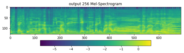
D = librosa.stft(
output_256,
n_fft=fft_size,
hop_length=hop_size,
win_length=win_length,
window=window,
pad_mode='reflect',
)
S, _ = librosa.magphase(D)
mel = np.log10(np.maximum(np.dot(mel_basis, S), 1e-10)).T
fig = plt.figure(figsize=(10, 8))
ax1 = fig.add_subplot(311)
ax1.set_title('output 256 Mel-Spectrogram')
im = ax1.imshow(np.rot90(mel), aspect='auto', interpolation='none')
fig.colorbar(mappable=im, shrink=0.65, orientation='horizontal', ax=ax1)
plt.show()
[22]:
D = librosa.stft(
output_128,
n_fft=fft_size,
hop_length=hop_size,
win_length=win_length,
window=window,
pad_mode='reflect',
)
S, _ = librosa.magphase(D)
mel = np.log10(np.maximum(np.dot(mel_basis, S), 1e-10)).T
fig = plt.figure(figsize=(10, 8))
ax1 = fig.add_subplot(311)
ax1.set_title('output 128 Mel-Spectrogram')
im = ax1.imshow(np.rot90(mel), aspect='auto', interpolation='none')
fig.colorbar(mappable=im, shrink=0.65, orientation='horizontal', ax=ax1)
plt.show()

[23]:
D = librosa.stft(
y_,
n_fft=fft_size,
hop_length=hop_size,
win_length=win_length,
window=window,
pad_mode='reflect',
)
S, _ = librosa.magphase(D)
mel = np.log10(np.maximum(np.dot(mel_basis, S), 1e-10)).T
fig = plt.figure(figsize=(10, 8))
ax1 = fig.add_subplot(311)
ax1.set_title('interpolate Mel-Spectrogram')
im = ax1.imshow(np.rot90(mel), aspect='auto', interpolation='none')
fig.colorbar(mappable=im, shrink=0.65, orientation='horizontal', ax=ax1)
plt.show()
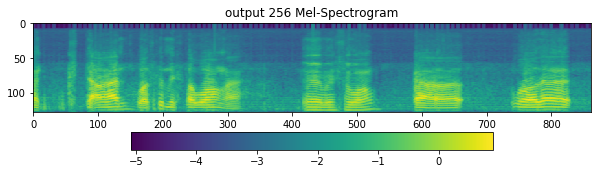
Try more examples#
[24]:
y, sr_ = malaya_speech.load('speech/call-centre/1.wav', sr = sr // reduction_factor)
y = y[sr_ * 5 :sr_ * 10]
sr_
[24]:
11025
[25]:
ipd.Audio(y, rate = sr_)
[25]:
[26]:
%%time
output = model(y)
ipd.Audio(output, rate = sr)
CPU times: user 30.1 s, sys: 3.39 s, total: 33.5 s
Wall time: 5.52 s
[26]:
[30]:
D = librosa.stft(
output,
n_fft=fft_size,
hop_length=hop_size,
win_length=win_length,
window=window,
pad_mode='reflect',
)
S, _ = librosa.magphase(D)
mel = np.log10(np.maximum(np.dot(mel_basis, S), 1e-10)).T
fig = plt.figure(figsize=(10, 8))
ax1 = fig.add_subplot(311)
ax1.set_title('output 256 Mel-Spectrogram')
im = ax1.imshow(np.rot90(mel), aspect='auto', interpolation='none')
fig.colorbar(mappable=im, shrink=0.65, orientation='horizontal', ax=ax1)
plt.show()
[31]:
%%time
output = model_128(y)
ipd.Audio(output, rate = sr)
CPU times: user 9.3 s, sys: 1.67 s, total: 11 s
Wall time: 1.95 s
[31]:
[33]:
D = librosa.stft(
output,
n_fft=fft_size,
hop_length=hop_size,
win_length=win_length,
window=window,
pad_mode='reflect',
)
S, _ = librosa.magphase(D)
mel = np.log10(np.maximum(np.dot(mel_basis, S), 1e-10)).T
fig = plt.figure(figsize=(10, 8))
ax1 = fig.add_subplot(311)
ax1.set_title('output 128 Mel-Spectrogram')
im = ax1.imshow(np.rot90(mel), aspect='auto', interpolation='none')
fig.colorbar(mappable=im, shrink=0.65, orientation='horizontal', ax=ax1)
plt.show()

[29]:
y_ = malaya_speech.resample(y, sr_, sr)
ipd.Audio(y_, rate = sr)
[29]:
[34]:
D = librosa.stft(
y_,
n_fft=fft_size,
hop_length=hop_size,
win_length=win_length,
window=window,
pad_mode='reflect',
)
S, _ = librosa.magphase(D)
mel = np.log10(np.maximum(np.dot(mel_basis, S), 1e-10)).T
fig = plt.figure(figsize=(10, 8))
ax1 = fig.add_subplot(311)
ax1.set_title('interpolate Mel-Spectrogram')
im = ax1.imshow(np.rot90(mel), aspect='auto', interpolation='none')
fig.colorbar(mappable=im, shrink=0.65, orientation='horizontal', ax=ax1)
plt.show()
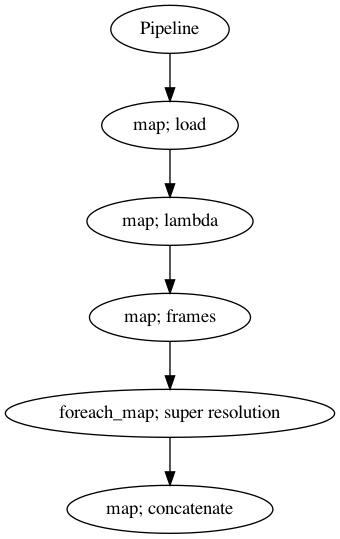
Use Pipeline#
Incase your audio is too long and you do not want to burden your machine. So, you can use malaya-speech Pipeline to split the audio splitted to 3 seconds, predict one-by-one and combine after that.
[20]:
p = Pipeline()
pipeline = (
p.map(malaya_speech.load, sr = sr // reduction_factor)
.map(lambda x: x[0])
.map(malaya_speech.generator.frames, frame_duration_ms = 3000, sample_rate = sr // reduction_factor)
.foreach_map(model_128)
.map(np.concatenate)
)
p.visualize()
[20]:
[21]:
%%time
results = p('speech/podcast/nusantara.wav')
CPU times: user 20.2 s, sys: 2.52 s, total: 22.7 s
Wall time: 4.19 s
[22]:
results.keys()
[22]:
dict_keys(['load', '<lambda>', 'frames', 'super-resolution', 'concatenate'])
[23]:
ipd.Audio(results['concatenate'], rate = sr)
[23]:
[24]:
ipd.Audio(results['<lambda>'], rate = sr // reduction_factor)
[24]:
[25]:
y_ = malaya_speech.resample(results['<lambda>'], sr // reduction_factor, sr)
ipd.Audio(y_, rate = sr)
[25]: